STS Walkthrough

Phase I: Bug Finding

We start by using STS to find bugs in controller software. STS supports two ways to accomplish this goal: most commonly, we use STS to simulate a network, generate random network events, and periodically check invariants; we also run STS interactively so that we can examine the state of any part of the simulated network, observe and manipulate messages, and follow our intuition to induce orderings that we believe may trigger bugs.

Fuzzing Mode

Fuzzing mode is how we use STS to generate randomly chosen input sequences in search of bugs. Let’s begin by looking at how we run the STS fuzzer.

In the config/ subdirectory, we find a configuration file fuzz_pox_simple.py we’ll use to specify our experiment.

The first two lines of this file tells STS how to boot the SDN controller (in this case, POX):

start_cmd = ('''./pox.py samples.buggy '''
             '''openflow.of_01 --address=__address__ --port=__port__''')
controllers = [ControllerConfig(start_cmd, cwd="pox/")]

Here we’re running a POX application with a known bug (samples.buggy). Note that the macros “__address__” and “__port__” are expanded by STS to allow it to choose available ports and addresses.

The next two lines specify the network topology we would like STS to simulate:

topology_class = MeshTopology
topology_params = "num_switches=2"

In this case, we’re simulating a simple mesh topology consisting of two switches each with an attached host, and a single link connecting the switches. For a complete list of default topologies STS supports (e.g. MeshTopology, FatTree), see the documentation. You might also consider using STS’s topology creation GUI to create your own custom topology:

$ ./simulator.py -c config/gui.py

The next line of our config file bundles up the controller configuration parameters with the network topology configuration parameters:

simulation_config = SimulationConfig(controller_configs=controllers,
                                     topology_class=topology_class,
                                     topology_params=topology_params)

The last line specifies what mode we would like STS to run in. In our case, we want to generate random inputs with the Fuzzer class:

control_flow = Fuzzer(simulation_config,
                      input_logger=InputLogger(),
                      invariant_check_name="InvariantChecker.check_liveness",
                      check_interval=5,
                      halt_on_violation=True)

Here we’re telling the Fuzzer to record its execution with an InputLogger, check every 5 fuzzing rounds whether the controller process has crashed, and halt the execution whenever we detect that the controller process has indeed crashed.

If the Fuzzer does not find a violation, it will continue running forever. To place on upper bound on how long it runs, we can add another parameter steps with a maximum number of rounds to execute, e.g. steps=500.

For a complete list of invariants to check, see the dictionary at the bottom of config/invariant_checks.py.

By default Fuzzer generates its inputs based on a set of event probabilities defined in config/fuzzer_params.py. Taking a closer look at that file, we see a list of event types followed by numbers in the range [0,1], such as:

 switch_failure_rate = 0.02
 switch_recovery_rate = 0.1
 ...

This tells the fuzzer to trigger kill live switches with a probability of 2%, and recover down switches with a probability of 10%.

Let’s go ahead and see STS in action, by invoking the simulator with our config file:

$ ./simulator.py -c config/fuzz_pox_simple.py

The output should look something like this:

console output

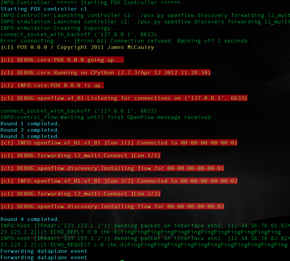
We see that STS populates the simulated topology, boots POX, connects the switches, and feeds in network traffic and other events. The console output is colored to delineate the different sources of output: the green output is STS’s internal logging, the blue output shows Fuzzer’s injected network events, and the orange output is the logging output of the POX controller process (“C1”).

One particularly useful feature of the Fuzzer is that you can drop into interactive mode, described next, by hitting ^C at any point in the execution. You can then return to Fuzzer by hitting ^D.

Interactive Mode

If you have a bug in mind, interactive mode is the perfect way to manually trigger it. It allows us to simulate the same network events as fuzzer mode, but gives us a command line interface to control the execution and examine the state of the network as we proceed.

We can run interactive either by hitting ^C during a fuzz execution, or by changing one line in the config file from before:

control_flow = Interactive(simulation_config, input_logger=InputLogger())

This tells STS to start with interactive mode rather than fuzzing. When we run STS with our modified configuration file, it will again populate the network topology, start the controller process, connect switches, and this time present us with a prompt:

console output

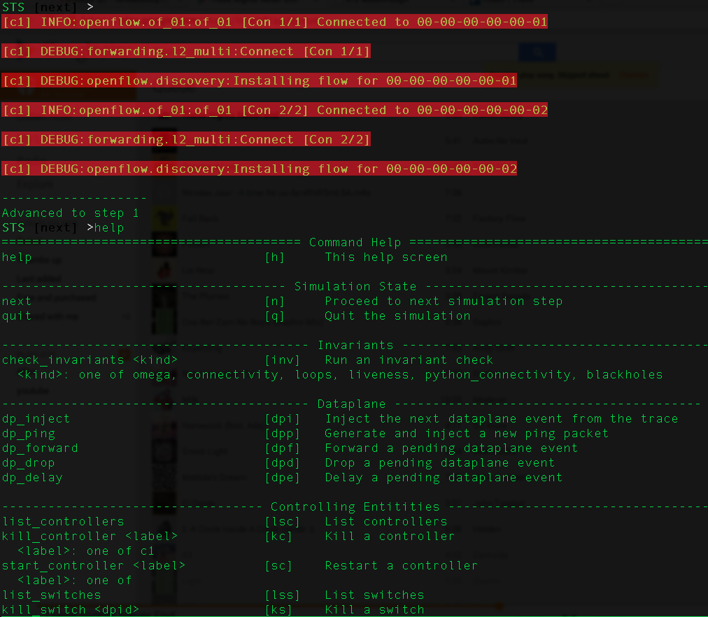
Each time we hit enter without other console input, the simulator will process any pending I/O operations (e.g. OpenFlow receipts), sleep for a small amount of time, and present us again with a prompt.

Interactive mode is particularly useful for examining the state of the network. For example, we can list all switches in the network by accessing the topology object’s switches property:

STS [next] >topology.switches
[SoftwareSwitch(dpid=1, num_ports=2), SoftwareSwitch(dpid=2, num_ports=2)]

We can also examine the current routing tables of a switch with the show_flows command:

STS [next] >show_flows 1
----------------------------------------------------------------------------------------------------------------------
|  Prio | in_port | dl_type | dl_src | dl_dst            | nw_proto | nw_src | nw_dst | tp_src | tp_dst | actions    |
----------------------------------------------------------------------------------------------------------------------
| 32768 |    None |    LLDP |   None | 01:23:20:00:00:01 |     None |   None |   None |   None |   None | CONTROLLER |
----------------------------------------------------------------------------------------------------------------------

From the prompt we can also check invariants, reorder or drop messages, and inject other network events such as link failures. Enter help for a full list of commands available in interactive mode.

Phase II: Troubleshooting

Let’s suppose we found a juicy invariant violation (if we let the Fuzzer run long enough, we should have eventually triggered a controller crash). Our InputLogger has recorded a trace of the network events that we can use to track down the root cause of the violation.

We can find the raw event trace in the experiments/fuzz_pox_simple directory:

$ ls experiments/fuzz_pox_simple/
__init__.py                  fuzzer_params.py             mcs_config.py     openflow_replay_config.py    replay_config.py
events.trace                 interactive_replay_config.py metadata          orig_config.py               simulator.out

The raw event trace is stored in the file events.trace. In this directory we find a number of other useful files: the simulator automatically copies your configuration parameters (fuzzer_params.py, orig_config.py), console output (simulator.out), metadata about the state of the system when the trace was recorded, and new configuration files for replaying the event trace (replay_config.py), minimizing the event trace (mcs_config.py), and root causing the bug (interactive_replay_config.py, openflow_replay_config.py).

By default, this experiments results directory is inferred from the name of the config file. You can also specify a custom name with the -n parameter to simulator.py. You can optionally specify that each experiment results directory should have a timestamp appended with the -t parameter.

The simplest way to start troubleshooting is by examining the event trace along with the console output. We rarely want to look at the event trace in its raw form though; we instead use a tool to parse and format the events:

$ ./tools/pretty_print_input_trace.py experiments/fuzz_pox_simple/events.trace
i1 ConnectToControllers (prunable)
fingerprint:  ()
--------------------------------------------------------------------
i2 ControlMessageReceive (prunable)
fingerprint:  (OFFingerprint{u'class': u'ofp_hello'}, 2, (u'c', u'1'))
...

The output of this tool is highly configurable; see the documentation for more information.

It is sometimes also helpful to group together similar classes of event types. We can accomplish this easily with another tool:

$ ./tools/tabulate_events.py experiments/fuzz_pox_simple/events.trace
====================== Topology Change Events ======================
e32 SwitchFailure (prunable)
fingerprint:  (1,)
--------------------------------------------------------------------
e58 SwitchRecovery (prunable)
fingerprint:  (1,)
--------------------------------------------------------------------
...

====================== Host Migration Events =======================
...

Replay Mode

Suppose we realize that we need to add more logging statements to the controller to understand what’s going on. With STS’s replayer mode, we can add our logging statements and then replay the same set of network events that triggered the original violation.

Replayer mode tries as best as it can to inject the network events from the trace in a way that reproduces the same outcome. It does this in part by maintaining the relative timing between input events as they appeared originally. Sometimes though the behavior of the controller can also change during replay. For example, the operating system may delay or reorder deliver of OpenFlow messages. For this reason STS also tracks the order and timing of internal events triggered by the controller software itself, and buffers these internal events during replay in an attempt to ensure the same causal order of events.

We can replay out trace simply by specifying replay_config.py as our configuration file:

$ ./simulator.py -c experiments/fuzz_pox_simple/replay_config.py
...
00:01.003 00:00.000 Successfully matched event ConnectToControllers:i1
00:01.006 00:00.000 Successfully matched event ControlMessageReceive:i2 c1 -> s2 [ofp_hello: ]
...

Like Fuzzer, we can drop into interactive mode at any time by sending ^C, and return to replay by sending ^D.

We can now replay as many times as we need to understand the root cause. The console output and other results from our replay runs can be found in a new subdirectory experiments/fuzz_pox_simple_replay/.

MCS Finder Mode

Randomly generated event traces often contain a large number of events, many of which distract us during the troubleshooting process and are not actually relevant for the bug we are interested in. In such cases we can attempt to minimize the original event trace, leaving just behind just the events that are directly responsible for triggering the bug.

STS’s MCSFinder mode executes the delta debugging algorithm to minimize the original event log. We can invoke MCSFinder by specifying the appropriate configuration file:

$ ./simulator.py -c experiments/fuzz_pox_simple/mcs_config.py

At the end of the console output, we should see a minimal sequence of inputs that are sufficient for triggering the original bug. In the case of POX’s buggy module, we see that a single SwitchFailure event is enough to cause the controller to crash.

The output of MCSFinder is yet another event trace that we can replay to continue with our troubleshooting. The results are stored in a new subdirectory experiments/fuzz_pox_simple_mcs/. The minimized event trace can be found in the mcs.trace and mcs.trace.notimeouts files. In addition, we see subdirectories such as interreplay_1_l_0/, which store results from intermediate replays throughout delta debugging’s execution. Finally, we can see statistics about MCSFinder’s progress by graphing the data stored in the runtime_stats.json file:

$ ./runtime_stats/generate_graph.py experiments/fuzz_pox_simple_mcs/runtime_stats.json

The resulting graph will show us the decreasing size of the event trace throughout the delta debugging’s execution:

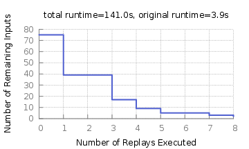
Root Causing

The last stage of the troubleshooting process involves understanding the precise circumstances that caused the controller software to err. STS includes several tools to help with this process.

InteractiveReplayer Mode

Sometimes Replayer moves too quickly to get a good understanding of an event trace. InteractiveReplayer is a combination of Interactive mode and Replayer mode, designed to help with:

visualizing the network topology
tracing the series of link/switch failures/recoveries
tracing the series of host migrations
tracing the series of flow_mods
tracing the series of traffic injections
tracing the series of controller failures, recoveries, and partitions

We can invoke InteractiveReplayer mode by invoking its automatically generated config file:

$ ./simulator.py -c experiments/fuzz_pox_simple/interactive_replay_config.py
STS [next] >
Injecting ControlMessageReceive:i2:(u'ControlMessageReceive', OFFingerprint{u'class': u'ofp_hello'}, 2, (u'c', u'1'))

Here we’re presented with another interactive prompt. Each time we hit enter, the next event in the trace is executed. We can also check invariants, examine flow tables, visualize the topology, and even induce previously unobserved inputs.

Because the timing of events is so delicate in a distributed system, InteractiveReplayer does not run controller processes. Instead, it mocks out OpenFlow connections, and replays the exact OpenFlow commands from the original trace.

OpenFlowReplayer Mode

The OpenFlow commands sent by controller software are often somewhat redundant. For example, flow_mods may override each other, expire, or periodically flush the contents of flow tables and later repopulate them. Hence even in minimized event traces we often observe OpenFlow messages that are not directly relevant for causing an invalid network configuration such as a loop or blackhole.

OpenFlowReplayer mode is designed to filter out such redundant messages, leaving only the flow_mods that show up in the final routing tables. With this knowledge, it becomes much easier to know exactly what points in the trace the invalid network configuration was installed.

Like the other modes, we can use OpenFlowReplayer mode simply by passing its config file as an argument to simulator.py:

$ ./simulator.py -c experiments/fuzz_pox_simple/openflow_replay_config.py
INFO:simulation:Creating topology...
Injecting ControlMessageReceive:i2:(u'ControlMessageReceive', OFFingerprint{u'class': u'ofp_hello'}, 2, (u'c', u'1'))
...

Filtered flow mods:
ControlMessageReceive:i19:(u'ControlMessageReceive', OFFingerprint{u'hard_timeout': 0, u'out_port': 65535, u'priority': 32768, u'idle_timeout': 0, u'command': u'add', u'actions': (u'output(65533)',), u'flags': 0, u'class': u'ofp_flow_mod', u'match': u'dl_dst:01:23:20:00:00:01,dl_type:35020'}, 1, (u'c', u'1'))
ControlMessageReceive:i32:(u'ControlMessageReceive', OFFingerprint{u'hard_timeout': 0, u'out_port': 65535, u'priority': 32768, u'idle_timeout': 0, u'command': u'delete', u'actions': (), u'flags': 0, u'class': u'ofp_flow_mod', u'match': u'x^L'}, 2, (u'c', u'1'))
...

Flow tables:
Switch 1
-------------------------------------------------------------------------------------------------------------------------------------------
|  Prio | in_port | dl_type |            dl_src |            dl_dst | nw_proto |      nw_src |      nw_dst | tp_src | tp_dst |    actions |
-------------------------------------------------------------------------------------------------------------------------------------------
| 32768 |    None |    LLDP |              None | 01:23:20:00:00:01 |     None |        None |        None |   None |   None | CONTROLLER |
| 32768 |    None |      IP | 12:34:56:78:01:02 | 12:34:56:78:01:02 |     ICMP | 123.123.1.2 | 123.123.1.2 |      0 |      0 |  output(2) |
-------------------------------------------------------------------------------------------------------------------------------------------
...

After replaying all OpenFlow commands, OpenFlowReplayer infers which flow_mods show up in the final routing tables.

Visualization tools

Understanding the timing of messages and internal events in distributed systems is a crucial part of troubleshooting. STS includes two visualization tools designed help with this task. First, the ./tools/visualization/visualize2d.html tool will show an interactive Lamport time diagram of an event trace:

$ open ./tools/visualization/visualize2d.html

A demo page is also available here.

After loading an event trace, we see a line for each switch, controller, and host in the network. If we hover over events, we can see more information about them. We can also adjust the size of the timeline by dragging our mouse up or down within the timeline area.

We include a second visualization tool, ./tools/visualization/visualize1d.html, to help us compare the behavior of two or more event traces. This tool is particularly useful for understanding the effects of non-determinism in intermediate runs of delta debugging.

A common workflow for the trace comparison tool:

Run MCSFinder.
Discover that the final MCS does not reliably trigger the bug.
Open visualize1D.html in a web browser.
Load either the original (fuzzed) trace, experiments/experiment_name/events.trace, or the first replay of this trace, experiments/experiment_name_mcs/interreplay_0_reproducibility/events.trace, as the first timeline. I have found that it is often better to load the first replay rather than the original fuzzed trace, since this has timing information that matches the other replays much more closely.
Load the final replay of the MCS trace, experiments/experiment_name_mcs/interreplay_._final_mcs_trace/events.trace, as the second timeline.
Hover over events to further information about them, including functional equivalence with events in the other traces.
Load intermediate replay trace timelines if needed. Intermediate replay traces from delta debugging runs can be found in experiments/experiment_name_mcs/interreplay_*

Tracing Packets Through the Network

It is often useful to know what path a packet took through the network. Given the event id of a TrafficInjection event, the ./tools/trace_traffic_injection.py script will print all dataplane permits and drops, as well as ofp_packet_in’s and out’s associated with the TrafficInjection’s packet:

$ ./tools/trace_traffic_injection.py experiments/fuzz_pox_simple/events.trace e22
e22 TrafficInjection (prunable)
fingerprint:  (Interface:HostInterface:eth2:12:34:56:78:02:02:[IPAddr('123.123.2.2')] Packet:[12:34:56:78:02:02>12:34:56:78:02:02:IP]|([v:4hl:5l:72t:64]ICMP cs:368c[123.123.2.2>123.123.2.2]){t:ECHO_REQUEST c:0 chk:637}{id:20585 seq:28263}, 2)
--------------------------------------------------------------------
i23 DataplanePermit (prunable)
fingerprint:  (DPFingerprint{u'dl_dst': u'12:34:56:78:02:02', u'nw_src': u'123.123.2.2', u'dl_src': u'12:34:56:78:02:02', u'nw_dst': u'123.123.2.2'}, 2, u'12:34:56:78:02:02')
--------------------------------------------------------------------
i28 ControlMessageSend (prunable)
fingerprint:  (OFFingerprint{u'data': DPFingerprint{u'dl_dst': u'12:34:56:78:02:02', u'nw_src': u'123.123.2.2', u'dl_src': u'12:34:56:78:02:02', u'nw_dst': u'123.123.2.2'}, u'class': u'ofp_packet_in', u'in_port': 2}, 2, (u'c', u'1'))
--------------------------------------------------------------------
...

Fin!

That’s it! See this page for a deeper dive into the structure of STS’s code, including additional configuration parameters to STS’s different modes. For an overview of how to generate dataplane traffic in STS, see this page. Finally, you should check out our collection of replayable experiments that have been used to find and troubleshoot real bugs in SDN controllers:

$ git clone git://github.com/ucb-sts/experiments.git

Questions?

Send questions or feedback to: sts-dev@googlegroups.com